Staying Connected and Entertained while Social Distancing

Staying Connected and Entertained while Social Distancing

Context: Coronavirus

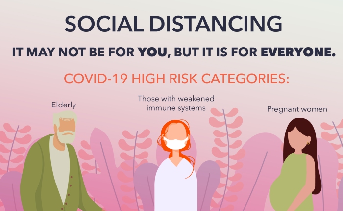
Unless your from another planet or just returned from a long solitary meditation retreat (like actor, Jared Leto), you have likely been asked to take several precautions in the face of this novel coronavirus (also referred to as Covid-19 and SARS-CoV-2) outbreak, which has been characterized as a pandemic by the World Health Organization as of March 11, 2020. The situation remains dire and Legislators around the world are asking us to each do our part in minimizing the spread of the virus.  Visit the CDC’s website for the latest recommendations on ways to prevent the spread and measures to take if you think you’ve been exposed.

Ideas to stay safe, connected, and entertained

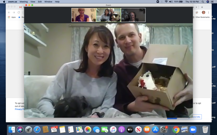
Since the grim news about the infection rate, mortality rate, and social and economic toll (e.g., Washington PostVox; CNN; fivethirtyeight; NPR) is being thoroughly covered by the media, I thought I would follow the lead of my mother-in-law and fellow blogger, Yvette Francino, in sharing ideas for safely socializing, up-skilling, volunteering, donating and staying healthy and entertained during the outbreak. Before you go through my list, I highly recommend that you look through her list of great ideas, which you can read on her blog (full disclaimer: I am featured on her blog because I celebrated my birthday virtually through the meeting app, Zoom):

Zoom Birthday Celebration because of the Coronavirus
Celebrating my birthday virtually over the meeting app Zoom with my family because of the coronavirus (also referred to as SARS-CoV-2 or Covid-19). Credit: Yvette Francino

Socialize

Virtual Meetings for 3+ people

  • Zoom works on most devices (e.g., Mac, Windows, Linux) and offers a free basic plan. One thing to note is that if you sign up for the free tier, your meetings are limited to 40 minutes if there are 3+ participants meetings a with the max number of participants capped at 100. There are no time caps for 1:1 meetings. If you are a K-12 educator, Zoom is currently offering you access to their platform for free (see this Forbes article for details).
  • Skype also works on most devices and offers a free plan. It’s unclear whether Skype allows multiple participants.
  • Google Hangouts also works on most devices and is free, with a Google account. You can host up to 10 people under the free plan.

Stay Entertained

Gaming Platforms

  • Steam is a popular game distributor that works on Windows, Mac, Linux, and mobile devices. They have some games that are available for free but most games are not free. Some of my favorites are the Jackbox Party series, which you can play with friends by hosting a game on one of the virtual meeting apps I listed above. Note that to play the Jackbox games virtually with your friends, they’ll need two devices: one for the meeting app to view the shared screen and another to play the games (they recommend a mobile device).
  • Origin is another popular gaming platform that works on most devices and offers free games but most games are not free.

Not a gamer but enjoy watching others play games? Then there’s always Twitch. You can also watch and support artists and musicians on Twitch as well (e.g. musicians channel).

Virtual Concerts & Tours

Read

or listen to a free audio book from LibriVox.

Stay Healthy

Exercise

  • Practice yoga for free with great YouTube instructors like Sara Beth who has 10-60 minute videos on different types of practices with modifications to accommodate all skill levels and abilities. You can also pay for platforms like CorePower Yoga.
  • Several studios are also streaming free fitness classes online, like LifeTime Fitness, YMCA360, Blink Fitness and Planet Fitness, or cardio dance classes like 305 Fitness.

Mental Health

  • Breathe2Relax is a free stress management app for iOS and Android that was developed by the U.S. Department of Veterans Affairs for anyone coping with trauma and anxiety. The VA has also developed other free apps that you may enjoy as well, like the Mindfulness app.
  • 7 Cups for iOS and Android is a free app that connects you to caring listeners for emotional support. They also provide online therapy for as little as $150 a month.
  • Talkspace for iOS and Android is an app that connects you with licensed therapists. They have multiple pricing tiers that range from $260 a month to $396 a month. They also offer couples therapy. More information on pricing here.
  • BetterHelp is an online text-based or chat-based counseling platform that connects you to therapists that specialize in individuals, couples, and adolescents. They charge between $40 to $70 per week.
  • Gottman Apps for iOS and Android is a free app developed by clinical psychologists, John and Julie Schwartz Gottman, and designed for couples.
  • Calm is a free mediation app for iOS and Android devices. Headspace for iOS and Android is a guided meditation app. It’s available by subscription only and costs $12.99 a month or you can pay $95.88 for the full year.

If you’re in serious crisis, you can always call the Suicide Prevention Lifeline, toll-free, at 1-800-273-8255.

Learn

Helping others if you can

If you’re healthy and able, also consider helping others by:

  • Picking up a few shifts at a local grocery store or distribution center and delivering food to support local businesses and their employees who are trying to keep their doors open, shelves stocked, and make sure people are fed.
  • Donating blood to organizations like the Red Cross. According to their website, we’re currently facing “a severe blood shortage due to an unprecedented number of blood drive cancellations during this coronavirus outbreak.” Make an appointment here or call 1-800-RED-CROSS to find a local donation site.
  • Donating funds to No Kid Hungry, which is an organization that ensures that millions of young children get access to food while schools are closed. You can also donate money, food, or hygiene items to Feed the Children, which partners with food pantries, soup kitchens, churches, and shelters around the country. There’s also Feeding America, which is a nationwide network of 200 food banks and 60,000 food pantries that serve vulnerable communities of children and adults across the country (find your local food bank here).
  • Donating to nonprofit organizations like Direct Relief or Center for Disaster Philanthropy Covid-19 Response Fund, which help to equip the amazing healthcare workers and service providers across the country that are putting themselves at risk everyday with lifesaving resources like masks, gloves, and gowns.
  • Donating or volunteering with Meals on Wheels, which is an organization that checks on vulnerable seniors, in addition to providing them with food, healthcare supplies, and transportation.
  • Contribute to Covid-19 community funds to help local restaurant workers, artists, people in extreme poverty, and other community members that are facing economic hardship because of the outbreak.

There are many other wonderful charities out there that are doing amazing work. If you want to check if a charity that you’re interested in is one of them, I recommend researching them on GiveWell.

Please remember that even if you are unable to do any of the above, you are doing plenty enough by following the general suggested guidance of maintaining your distance from others (especially if you are sick)avoiding the urge to hoard, and staying informedBy maintaining your distance and avoiding public spaces, you’re saving lives by reducing the risk of transmission.

Thank you for doing your part! Please share your ideas in a comment below or through another medium like twitter or a blog to inspire others.


Gapminder gif with Rstudio

Gapminder gif with Rstudio

I decided to remake the Gapminder gif that I made the other day in Python, but in Rstudio this time. I’ll probably continue doing this for a while, as I try to figure out the advantages of using one program over the other. Here’s is a walk-through of what I did to recreate it:

#install these packages if you haven't already
install.packages(c("devtools", "dplyr", "ggplot2", "readr"))
devtools::install_github("dgrtwo/gganimate",force=TRUE)

library(devtools)
library(dplyr)
library(readr)
library(viridis)
library(ggplot2)
library(gganimate)
library(animation)

#Set up ImageMagick --for gifs
install.packages("installr",dependencies = TRUE)
library(installr)

#Configure your environment--change the location
Sys.setenv(PATH = paste("C:/Program Files/ImageMagick-7.0.7-Q16", Sys.getenv("PATH"), sep = ";")) #change the path to where you installed ImageMagick
#Again, change the location:
magickPath <- shortPathName("C:/Program Files/ImageMagick-7.0.7-Q16/magick.exe")
#ani.options(convert=magickPath)

If you need to download ImageMagick, go to this link

Load data and create plot

Once you’ve installed the appropriate packages and configured ImageMagick to work with Rstudio, you can load your data and plot as usual.

gapminder_data<-read.csv("https://python-graph-gallery.com/wp-content/uploads/gapminderData.csv", header=TRUE)

glimpse(gapminder_data) #print to make sure it loaded correctly
## Observations: 1,704
## Variables: 6
## $ country    Afghanistan, Afghanistan, Afghanistan, Afghanistan, ...
## $ year       1952, 1957, 1962, 1967, 1972, 1977, 1982, 1987, 1992...
## $ pop        8425333, 9240934, 10267083, 11537966, 13079460, 1488...
## $ continent  Asia, Asia, Asia, Asia, Asia, Asia, Asia, Asia, Asia...
## $ lifeExp    28.801, 30.332, 31.997, 34.020, 36.088, 38.438, 39.8...
## $ gdpPercap  779.4453, 820.8530, 853.1007, 836.1971, 739.9811, 78...
# Helper function for string wrapping. 
# Default 20 character target width.
swr = function(string, nwrap=40) {
  paste(strwrap(string, width=nwrap), collapse="\n")
}
swr = Vectorize(swr)

gapminder_plot<-ggplot(gapminder_data) +
  aes(x = gdpPercap,
      y = lifeExp,
      colour = continent,
      size = pop, 
      frame=year) +
      scale_x_log10() +
  scale_size_continuous(guide =FALSE) + #suppresses the second legend (size=pop)
  geom_point() +
  scale_color_viridis(discrete=TRUE)+ #optional way to change colors of the plot
  theme_bw() +
  labs(title=swr("Relationship Between Life Expectancy and GDP per Capita"),
       x= "GDP Per Capita",
       y= "Life expectancy",
      caption="Data: Gapminder")
  theme(legend.position = "none",
        axis.title.x=element_text(size=.2),
        axis.title.y=element_text(size=.2),
        plot.caption = element_text(size=.1))</

#getOption("device") #try running this if your plot doesn't immediately show gapminder_plot

#if you want to save the plot:
ggsave("title.png", 
       plot = last_plot(), # or give ggplot object name as in myPlot,
       width = 5, height = 5, 
       units = "in", # other options c("in", "cm", "mm"), 
       dpi = 300)

Notice that I created the swr function to wrap the title text. If I don’t include that function, the title runs off the plot, like this:

gapminderplot

Animate the plot

Now you can animate the plot using gganimate. Also, if you want to change any of the axis-titles or any other feature of the plot, I like to reference STHDA.

#remember to assign a working directory first:
#setwd() <--use this to change the working directory, if needed
gganimate(gapminder_plot,interval=.5,"gapminderplot.gif")


All in all, I’d say that creating the gif was equally easy in Python and R. Although I had more trouble initally configuring Python with ImageMagic–I might have found it easier in R simply because I used Python to figure this out the first time.  On the other hand, I like the way the Python gif looks much more than the gif that Rstudio rendered.

animated_gapminder

Looks like I’ll have to continue experimenting.

OLS Tutorial in Stata Cont.

This post is an addendum to the OLS tutorial I posted two weeks ago. I will walk through the explanations that I provided in the program and I will interpret the output. If you haven’t read the previous post, you can access the materials using this link.

The tutorial begins by telling the user to run the following two lines of code:

clear all

set more off, permanently

The “clear” command will clear out data, along with any value labels, that are currently loaded in Stata. The additional command “all” will clear matrices, scalars,
constraints, clusters, stored results, sersets, and Mata functions and objects from the memory, in addition to closing all open files and postfiles, clear the class system, close any open Graph windows and dialog boxes, drop all programs from memory, and reset all timers to zero.

The next command, “set more off,” changes Stata’s default setting, which is “set more on.” The “set more off” command tells Stata not to pause or display the ” –more–” message when showing results. Personally, I hate pressing spacebar over and over again until all of my results are displayed.  Stata will make “set more off” the new default by adding the option (noted by the “,”) “permanently.” Note that once you run this command, you do not have to run it again, now that “set more off” is the default. You can change this back by typing “set more on, permanently”. You can read more about the clear function here and the set more off function here.

In the next step, the tutorial directs you to load your data:

use “[folder path data is in]\[datafile name]”

I stored my data in the folder “C:\Users\Stella\Documents\blog\ols”. This should be put in place of the text:”[folder path data is in]”, including the brackets. The file name is “nlsy97_2015”. This should be put in the place of the text: “[datafile name]”, including brackets, such that the final will read:

use “C:\Users\Stella\Documents\blog\ols\nlsy97_2015”

You could add the option “,clear” to this instead of using the “clear all” command above, and it would effectively accomplish the same thing.

Next, I walk through how to set up a log file. A log records your Stata session. You can run multiple logs at the same time if you wish. It’s nice to keep a log of your work so that you can track what syntax was used to generate your output. In the program, I store the log in the same folder as my data. I name my log SMnlsy97_2015.txt. I add the option “replace” to allow Stata to write over an existing log, if there is one. You generally want to do this because it is likely that you will make mistakes and have to re-run your program.

In the next section of the program, I walk you through commands that allow you to look at your variables. For example, I look at the variable Wage, which is the outcome variable in this tutorial:

codebook Wage

This will produce the following output:

codebook

As you can see, codebook will show you information about the variable, such as the type of variable it is (numeric), the lowest value (0) and highest value (110,000), the number of unique values (400), the number of missing values (1400), the mean (40209), the standard deviation (27211.2), and the interquartile range. If you ran the command “codebook” without specifying a variable or variables, it would produce output for every variable in the dataset.

You can view a summary of the variable by typing:

summarize Wage, detail

For short, you can type “sum” in the place of summarize and “d” in the place of detail. This command should produce the following output:

sum

The output confirms some of the details we saw using codebook: The smallest value for Wage is $0, while the largest is $110,000; the mean wage is $40,209.03, with a standard deviation of $27.211.23. Unlike codebook, summarize shows us that there are 5,702 observations for the variable Wage; the median value, represented by the 50th percentile, is $36,000; and we can now see that the data is skewed. The value associated “skewness” tells us the degree and direction in which the data is skewed, which is skewed to the right (indicated by the positive value). Note that we can tell that the variable is skewed because the mean exceeds the median. Kurtosis is a measure of how heavily the data is skewed–heavily skewed data will show a value greater than 3. See UCLA IDRE for a detailed explanation.

You can view a visual representation of the variable by creating a histogram:

histogram Wage, normal

histogram

The “normal” option produces a bell curve that approximates what a normal distribution would look like. You can see that the distribution of Wage is not normally distributed. The bars spike above the curve and fall far below the curve throughout the distribution of wage Values (x-axis). Then you can see that there is a sudden spike again in the tail around the wage $150,000, where I top coded the wages.

It is generally expected that you run descriptive statistics on all of your variables. More on this in a second. First, you should check your variables for missing observations. There are several ways to do this. One way to do this is with the command misstable summarize. Note that you can specify which variables to look at (e.g., misstable summarize variable1 variable2…). By default, the command will look at all variables in the data. In the case of these data, that is okay because I’ve shortened the dataset to contain less than 20 variables. The result should be this:

misstable

You should see the variables that have missing observations, and the number of observations that are missing. For example, the variable mar_stat has 161 missing observations, whereas the variable biokids has 2,331. The table also reveals the number of unique values associated with each variable, along with the min and max values. The latter results can be observed in the summary table or if you use the command “tabulate”, which will produce frequency tables.

Another way to do this is with the command “mdesc”, which is a user-submitted command that tells Stata to generate a table that shows the missing values:

mdesc

The screen capture doesn’t show the results for all of the variables because it is cut off in my screen, but you get the idea. Again, by default, mdesc will run through all the variables in the dataset, unless you specify certain variables. Instead of showing you the number of unique values, and the lowest and highest values, mdesc shows you the percent that are missing, in addition to the total number of missing observations. I generally find this more helpful than the results produced by misstable summarize.

Next, I walk through different ways to address missing values. In the class that I made this tutorial for, replacing the missing values with the mean or mode was acceptable, as long as the student explicitly stated so. More advanced users will likely use methods such as multiple imputation (e.g., Stata13 Manual). You can also listwise delete any observations that contain missing values. I provide an example of a loop that will do this:


foreach

Most users find this confusing, so bear with me. The command says that “foreach” variable represented by some letter or word–in this case “v’–of the following varlist (aka “var”) *–which is short hand for all variables in this data. Stata is going to drop the observation if it missing. For example, the first variable in the example data is id. Stata will go through id and see if any of the values are missing. No values of id are missing, so Stata will go to the next variable (birth_month) and check for missing variables, and so on. When Stata gets to mar_stat, Stata will see that 161 people did not report their marital status, so Stata will remove them from the data, which will reduce our sample down to  6,941 observations (7,102-161). Then Stat will remove 2,331 observations for missing data on the number of biological children that they have, and so forth. In the end, you should have 3,623 observations. You can check this by running mdesc again.

Side note: Sometime in the future, I will provide a tutorial on loops because it is huge time saver, and it’s something that is not often taught in statistics courses (at least not in any of mine).

Continuing on with the tutorial, in the next section, I show the user how to generate formatted tables with a user-submitted command “estout”:

ssc install estout

You can add the option “replace” to update estout, if you’ve already installed the command. You can read more about the command by visiting this link. Now type the following:

estpost sum *

esttab usingC:\Users\Stella\Documents\blog\ols\OLSdescripts.rtf”, replace ///
cell((mean(label(Mean/Perc.) fmt(%9.2f)) sd(par label(S.D.) fmt(%9.2f)))) label nonumber nomtitle

eststo clear

The command “estpost” will show the results associated with whatever function you tell Stata to run on the data, in this case, I requested a summary of all my variables, as indicated by the asterisk (*). It will produce the following output:

estpost

The first column shows you the number of observations; the second shows the summary of weights (i.e., nonmissing observations); the third column shows you the mean of each variable; the fourth shows the variance; the fifth shows the standard deviation; the sixth shows the minimum value; the seventh shows the maximum value; and the last shows the sum of the variable. For descriptive statistics, we are interested in are: the mean, standard deviation, and the total number of observations. We use this information specifically in the next command which tells Stata to create a table (esttab) using this file location (C:\Users\Stella\Documents\blog\ols\) and this file name (OLSdescripts.rtf). I specify .rtf (rich text format) because I want to preserve the format. I use the option replace because I want to replace any existing document with this name. If you do not want to do this, simply change the name of the document (for example, OLSdescript2.rtf). Next, I tell Stata that I want the first cell (i.e., column) to display the mean, which should be labeled “Mean/Perc.” The label will be right justified and the numbers will show include two decimal places. The next cell/column will display the standard deviation, labeled as “S.D.” with the same formatting constraints. The next label option tells Stata that you want the labels associated with each variable, and to avoid adding the additional model number over each column that esttab adds by default. You should get the following output

TableNote that not all of the variables are labeled. You will want to do this before you submit an assignment or use the table in a research paper.

You can also use esttab to generate formatted regression tables:

OLSI show you how to do this toward the end of the program, after I go through quick explanations of how to check basic OLS assumptions.

A final note about the formatted results. Although esttab is a quick and easy way to create formatted tables within Stata, the user-submitted command tabout will give you even more control over how your results are displayed, especially if you know how to use LaTex. I spent a lot of time tinkering with LaTex and I never mastered it. Maybe a project for the future.

OLS Regression in Stata

I thought I would share some Stata programming files that I made for some students who were struggling with coding in a statistics course. The program covers OLS regression in Stata and references (mostly 2015) data from the National Longitudinal Study of Youth 1997 (NLSY97).  You can access the Stata programs and data set that I created from the Open Science Framework, using this link. I also included all of the original files, and a program that shows you how I coded the data set that is referenced for this tutorial.

The program assumes that the user has some basic Stata coding knowledge, such as coding variables, loading and saving data, and generating descriptive statistics. The program also does not cover how to interpret the results from the OLS regression. Instead, the program mostly focus on exporting descriptive statistics and OLS regression results to formatted tables within Word. They also describe in detail, how to conduct sensitivity analyses on the results. The reason I do not spend time explaining how to interpret the results is because there are already a ton of websites that do a great job of this; for example, see this detailed explanation at IDRE at UCLA. Instead, I offer ways to speed up the user’s productivity by exporting pre-formatted tables and I also provide a supplemental explanation of what the syntax is doing. This way, new users will not get hung up on learning to code in Stata, but instead, focus on learning more about the statistical concepts they are practicing.

For example, I provide comments after almost every line to explain what the syntax does specifically. I also walk the user through how to load data and save a log, which will also show the results of any model that the user runs. The reason why I specifically include explanations such as “[folder path data is in]\ [datafile name]” is because I found that some students were not familiar with what this line was doing. 

Pic1

For users who are not familiar with folder locations on the computer, you will have to include an additional step: showing how to copy and paste the folder path into the Stata program (illustrated by the highlighted folder address in the image below):

folderpath

When you are very comfortable with a computer, it’s easy to forget sometimes that this may be a totally foreign concept to someone who does not understand folder locations in a computer, which is a serious barrier to keeping up in statistics courses.

Basically, if the course is about programming in Stata, then of course, students should go through the steps for learning the syntax. If the course is about statistical concepts, and does focus on teaching the basics of programming, then I think it is important to provide more detailed explanations of what the syntax is doing.

With that said, the program that I provided is not perfect, but it certainly goes further than the typical explanation a student receives in a statistics course. I hope to improve it as I receive feedback from others. If you have any suggestions in how to do this, please let me know! Also, please feel free to share it with others or use it in your class, if you find it useful.