Plotly 3.0.0 in Jupyter Notebook

Plotly 3.0.0 in Jupyter Notebook

Plotly.py 3.0.0 was recently released, and I finally got a chance to tinker with it! This is exciting because this release includes features that are specifically designed for Jupyter Notebooks. Namely, JavaScript is directly embedded in the figure that you can now access directly through your notebook. Exciting!

If you haven’t installed plotly or need to upgrade, open your Anaconda command prompt (as Administrator) and follow these directions. After you install plotly, launch Jupyter Notebook (by typing “Jupyter Notebook” into your Anaconda command prompt or by opening Jupyter Notebook using your computer menu). Next, enter your plotly username and api key in your notebook. You can sign up for plotly here. Directions for generating an api key here.

#first import plotly and provide username and api key
import plotly
plotly.tools.set_credentials_file(username='UserName', api_key='XXXXX')

Now load the following:

import plotly.plotly as py
import plotly.graph_objs as go
from plotly.offline import download_plotlyjs, init_notebook_mode, plot, iplot
import numpy as np
import pandas as pd

init_notebook_mode(connected=True) #tells the notebook to load figures in offline mode

Plotly should now work within your notebook.

Here’s an example of a 2D plot:

x=np.random.randn(1000)
y=np.random.randn(1000)
go.FigureWidget(
    data=[
        {'x': x, 'y': y, 'type': 'histogram2dcontour'}
    ]
)

newplotExample of a 2D plot with markers:

x = np.random.randn(2000)
y = np.random.randn(2000)
iplot([go.Histogram2dContour(x=x, y=y, contours=dict(coloring='heatmap')),
       go.Scatter(x=x, y=y, mode='markers', marker=dict(color='white', size=3, opacity=0.3))], show_link=False)

newplot(1)
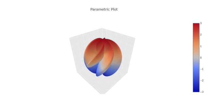
Example of a 3D plot:

s = np.linspace(0, 2 * np.pi, 240)
t = np.linspace(0, np.pi, 240)
tGrid, sGrid = np.meshgrid(s, t)

r = 2 + np.sin(7 * sGrid + 5 * tGrid)  # r = 2 + sin(7s+5t)
x = r * np.cos(sGrid) * np.sin(tGrid)  # x = r*cos(s)*sin(t)
y = r * np.sin(sGrid) * np.sin(tGrid)  # y = r*sin(s)*sin(t)
z = r * np.cos(tGrid)                  # z = r*cos(t)

surface = go.Surface(x=x, y=y, z=z)
data = [surface]

layout = go.Layout(
    title='Parametric Plot',
    scene=dict(
        xaxis=dict(
            gridcolor='rgb(255, 255, 255)',
            zerolinecolor='rgb(255, 255, 255)',
            showbackground=True,
            backgroundcolor='rgb(230, 230,230)'
        ),
        yaxis=dict(
            gridcolor='rgb(255, 255, 255)',
            zerolinecolor='rgb(255, 255, 255)',
            showbackground=True,
            backgroundcolor='rgb(230, 230,230)'
        ),
        zaxis=dict(
            gridcolor='rgb(255, 255, 255)',
            zerolinecolor='rgb(255, 255, 255)',
            showbackground=True,
            backgroundcolor='rgb(230, 230,230)'
        )
    )
)

fig = go.Figure(data=data, layout=layout)
py.iplot(fig, filename='jupyter-parametric_plot')
newplot(2)
Interact with it here

Lastly, an animated plot:

from plotly.offline import init_notebook_mode, iplot
from IPython.display import display, HTML


init_notebook_mode(connected=True)

url = 'https://raw.githubusercontent.com/plotly/datasets/master/gapminderDataFiveYear.csv'
dataset = pd.read_csv(url)

years = ['1952', '1962', '1967', '1972', '1977', '1982', '1987', '1992', '1997', '2002', '2007']


# make list of continents
continents = []
for continent in dataset['continent']:
    if continent not in continents:
        continents.append(continent)
# make figure
figure = {
    'data': [],
    'layout': {},
    'frames': []
}

# fill in most of layout
figure['layout']['xaxis'] = {'range': [30, 85], 'title': 'Life Expectancy'}
figure['layout']['yaxis'] = {'title': 'GDP per Capita', 'type': 'log'}
figure['layout']['hovermode'] = 'closest'
figure['layout']['sliders'] = {
    'args': [
        'transition', {
            'duration': 400,
            'easing': 'cubic-in-out'
        }
    ],
    'initialValue': '1952',
    'plotlycommand': 'animate',
    'values': years,
    'visible': True
}
figure['layout']['updatemenus'] = [
    {
        'buttons': [
            {
                'args': [None, {'frame': {'duration': 500, 'redraw': False},
                         'fromcurrent': True, 'transition': {'duration': 300, 'easing': 'quadratic-in-out'}}],
                'label': 'Play',
                'method': 'animate'
            },
            {
                'args': [[None], {'frame': {'duration': 0, 'redraw': False}, 'mode': 'immediate',
                'transition': {'duration': 0}}],
                'label': 'Pause',
                'method': 'animate'
            }
        ],
        'direction': 'left',
        'pad': {'r': 10, 't': 87},
        'showactive': False,
        'type': 'buttons',
        'x': 0.1,
        'xanchor': 'right',
        'y': 0,
        'yanchor': 'top'
    }
]
#custom colors
custom_colors = {
    'Asia': 'rgb(171, 99, 250)',
    'Europe': 'rgb(230, 99, 250)',
    'Africa': 'rgb(99, 110, 250)',
    'Americas': 'rgb(25, 211, 243)',
    'Oceania': 'rgb(50, 170, 255)'
}
sliders_dict = {
    'active': 0,
    'yanchor': 'top',
    'xanchor': 'left',
    'currentvalue': {
        'font': {'size': 20},
        'prefix': 'Year:',
        'visible': True,
        'xanchor': 'right'
    },
    'transition': {'duration': 300, 'easing': 'cubic-in-out'},
    'pad': {'b': 10, 't': 50},
    'len': 0.9,
    'x': 0.1,
    'y': 0,
    'steps': []
}

# make data
year = 1952
for continent in continents:
    dataset_by_year = dataset[dataset['year'] == year]
    dataset_by_year_and_cont = dataset_by_year[dataset_by_year['continent'] == continent]

    data_dict = {
        'x': list(dataset_by_year_and_cont['lifeExp']),
        'y': list(dataset_by_year_and_cont['gdpPercap']),
        'mode': 'markers',
        'text': list(dataset_by_year_and_cont['country']),
        'marker': {
            'sizemode': 'area',
            'sizeref': 200000,
            'size': list(dataset_by_year_and_cont['pop'])
        },
        'name': continent
    }
    figure['data'].append(data_dict)
    
# make frames
for year in years:
    frame = {'data': [], 'name': str(year)}
    for continent in continents:
        dataset_by_year = dataset[dataset['year'] == int(year)]
        dataset_by_year_and_cont = dataset_by_year[dataset_by_year['continent'] == continent]

        data_dict = {
            'x': list(dataset_by_year_and_cont['lifeExp']),
            'y': list(dataset_by_year_and_cont['gdpPercap']),
            'mode': 'markers',
            'text': list(dataset_by_year_and_cont['country']),
            'marker': {
                'sizemode': 'area',
                'sizeref': 200000,
                'size': list(dataset_by_year_and_cont['pop'])
            },
            'name': continent
        }
        frame['data'].append(data_dict)

    figure['frames'].append(frame)
    slider_step = {'args': [
        [year],
        {'frame': {'duration': 300, 'redraw': False},
         'mode': 'immediate',
       'transition': {'duration': 300}}
     ],
     'label': year,
     'method': 'animate'}
    sliders_dict['steps'].append(slider_step)

    
figure['layout']['sliders'] = [sliders_dict]

iplot(figure)
newplot(3)
Interact with it here

Neat, right?!


Overall, everything ran smoothly except the last plot. I actually initially tried to make this one:

gapminder_custom
From: https://plot.ly/python/gapminder-example/ (scroll to the bottom)

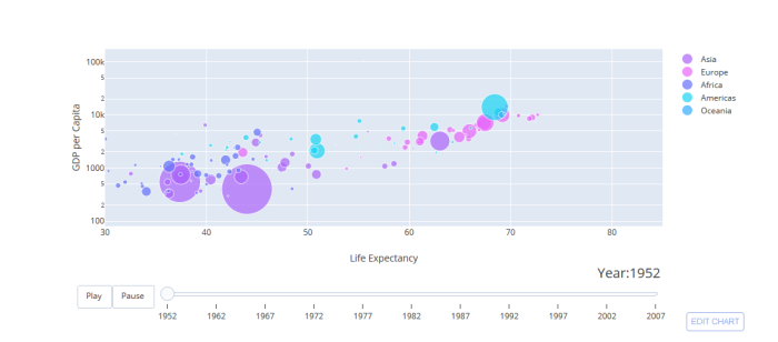
but I kept getting an error:

error

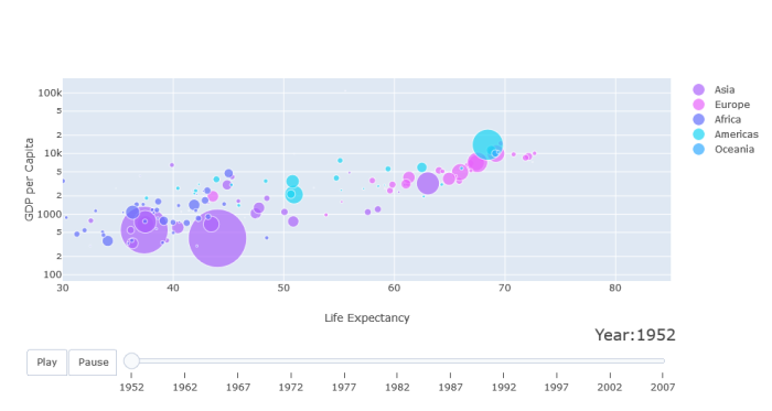
Update: Jon commented and pointed out that I was using an older version of plotly (3.0.0rc10) instead of 3.0.0rc11. You can check which version you have by typing the following:

import plotly
plotly.__version__

After I updated plotly, I successfully made the last graph!

newplot(4)
Interact with it here

Special thanks to Jon! I sincerely appreciate your help!

Understanding Linear Regression

My husband and I were discussing the intuition behind OLS regression today and I decided to share the materials that I generated to break down covariance, correlations, and the linear regression equation. It may help to follow along in the Excel workbook that I did this in (see link).

First, let’s say that we have the following data:

Y X1 X2
1 40 25
2 45 20
1 38 30
3 50 30
2 48 28
3 55 30
3 53 34
4 55 36
4 58 32
3 40 34
5 55 38
3 48 28
3 45 30
2 55 36
4 60 34
5 60 38
5 60 42
5 65 38
4 50 34
3 58 38

We plot the relationship between each X variable and Y, to get a visual look at their relationships:

x1y

x2y

I also like to look at the relationship in a 3D plot (this plot was made in Rstudio with plotly–see link for tutorial):

//plot.ly/~allets/6.embed

To calculate the mean of these data, we would have to sum each column and divide each column by the total number of observations (n=20):

Sum 65 1038 655
N 20 20 20
Mean 3.25 51.9 32.75

Now we need the standard deviation. This is something most students do not find very intuitive unless you force them to calculate this step by step, either by hand or in Excel. You should start by subtracting each observation in each column by it’s respective mean:

(Y-MeanY) (X1-MeanX1) (X2-MeanX2)
1-3.25=-2.25 40-51.9=-11.9 25-32.75=-7.75
2-3.25=-1.25 45-51.9=-6.9 20-32.75=-12.75
1-3.25=-2.25 38-51.9=-13.9 30-32.75=-2.75
3-3.25=-0.25 50-51.9=-1.9 30-32.75=-2.75
2-3.25=-1.25 48-51.9=-3.9 28-32.75=-4.75
3-3.25=-0.25 55-51.9=3.1 30-32.75=-2.75
3-3.25=-0.25 53-51.9=1.1 34-32.75=1.25
4-3.25=0.75 55-51.9=3.1 36-32.75=3.25
4-3.25=0.75 58-51.9=6.1 32-32.75=-0.75
3-3.25=-0.25 40-51.9=-11.9 34-32.75=1.25
5-3.25=1.75 55-51.9=3.1 38-32.75=5.25
3-3.25=-0.25 48-51.9=-3.9 28-32.75=-4.75
3-3.25=-0.25 45-51.9=-6.9 30-32.75=-2.75
2-3.25=-1.25 55-51.9=3.1 36-32.75=3.25
4-3.25=0.75 60-51.9=8.1 34-32.75=1.25
5-3.25=1.75 60-51.9=8.1 38-32.75=5.25
5-3.25=1.75 60-51.9=8.1 42-32.75=9.25
5-3.25=1.75 65-51.9=13.1 38-32.75=5.25
4-3.25=0.75 50-51.9=-1.9 34-32.75=1.25
3-3.25=-0.25 58-51.9=6.1 38-32.75=5.25

Then you will square each value in each column:

(Y-MeanY)^2 (X1-MeanX1)^2 (X2-MeanX2)^2
-2.25^2=5.0625 -11.9^2=141.61 -7.75^2=60.0625
-1.25^2=1.5625 -6.9^2=47.61 -12.75^2=162.5625
-2.25^2=5.0625 -13.9^2=193.21 -2.75^2=7.5625
-0.25^2=0.0625 -1.9^2=3.60999 -2.75^2=7.5625
-1.25^2=1.5625 -3.9^2=15.21 -4.75^2=22.5625
-0.25^2=0.0625 3.1^2=9.610000 -2.75^2=7.5625
-0.25^2=0.0625 1.1^2=1.21 1.25^2=1.5625
0.75^2=0.5625 3.1^2=9.610000 3.25^2=10.5625
0.75^2=0.5625 6.1^2=37.21 -0.75^2=0.5625
-0.25^2=0.0625 -11.9^2=141.61 1.25^2=1.5625
1.75^2=3.0625 3.1^2=9.610000 5.25^2=27.5625
-0.25^2=0.0625 -3.9^2=15.21 -4.75^2=22.5625
-0.25^2=0.0625 -6.9^2=47.61 -2.75^2=7.5625
-1.25^2=1.5625 3.1^2=9.610000 3.25^2=10.5625
0.75^2=0.5625 8.1^2=65.61 1.25^2=1.5625
1.75^2=3.0625 8.1^2=65.61 5.25^2=27.5625
1.75^2=3.0625 8.1^2=65.61 9.25^2=85.5625
1.75^2=3.0625 13.1^2=171.61 5.25^2=27.5625
0.75^2=0.5625 -1.9^2=3.60999 1.25^2=1.5625
-0.25^2=0.0625 6.1^2=37.21 5.25^2=27.5625

If you sum up each column of the squared values, you will get the standard deviation:

SD 29.75 1091.8 521.75

In addition to calculating the mean and standard deviation of Y, X1, and X2, you will also need to calculate the relationships between Y, X1, and X2 by first, multiplying them together, and then repeating each of the steps that we did above:

X1*Y X2*Y X1*X2
1*40=40 1*25=25 25*40=1000
2*45=90 2*20=40 20*45=900
1*38=38 1*30=30 30*38=1140
3*50=150 3*30=90 30*50=1500
2*48=96 2*28=56 28*48=1344
3*55=165 3*30=90 30*55=1650
3*53=159 3*34=102 34*53=1802
4*55=220 4*36=144 36*55=1980
4*58=232 4*32=128 32*58=1856
3*40=120 3*34=102 34*40=1360
5*55=275 5*38=190 38*55=2090
3*48=144 3*28=84 28*48=1344
3*45=135 3*30=90 30*45=1350
2*55=110 2*36=72 36*55=1980
4*60=240 4*34=136 34*60=2040
5*60=300 5*38=190 38*60=2280
5*60=300 5*42=210 42*60=2520
5*65=325 5*38=190 38*65=2470
4*50=200 4*34=136 34*50=1700
3*58=174 3*38=114 38*58=2204

Again, (1) sum each column and (2) divide by the total number of observations (n=20) to get the mean.

Sum 3513 2219 34510
N 20 20 20
Mean 175.65 110.95 1725.5

(3) In a separate table, subtract the respective mean for each column from each row value:

(X1*Y)-(MeanX1*Y) (X2*Y)-(MeanX2*Y) (X1*X2)-(MeanX1*X2)
40-175.65=-135.65 25-110.95=-85.95 1000-1725.5=-725.5
90-175.65=-85.65 40-110.95=-70.95 900-1725.5=-825.5
38-175.65=-137.65 30-110.95=-80.95 1140-1725.5=-585.5
150-175.65=-25.65 90-110.95=-20.95 1500-1725.5=-225.5
96-175.65=-79.65 56-110.95=-54.95 1344-1725.5=-381.5
165-175.65=-10.65 90-110.95=-20.95 1650-1725.5=-75.5
159-175.65=-16.65 102-110.95=-8.95 1802-1725.5=76.5
220-175.65=44.35 144-110.95=33.05 1980-1725.5=254.5
232-175.65=56.35 128-110.95=17.05 1856-1725.5=130.5
120-175.65=-55.65 102-110.95=-8.95 1360-1725.5=-365.5
275-175.65=99.35 190-110.95=79.05 2090-1725.5=364.5
144-175.65=-31.65 84-110.95=-26.95 1344-1725.5=-381.5
135-175.65=-40.65 90-110.95=-20.95 1350-1725.5=-375.5
110-175.65=-65.65 72-110.95=-38.95 1980-1725.5=254.5
240-175.65=64.35 136-110.95=25.05 2040-1725.5=314.5
300-175.65=124.35 190-110.95=79.05 2280-1725.5=554.5
300-175.65=124.35 210-110.95=99.05 2520-1725.5=794.5
325-175.65=149.35 190-110.95=79.05 2470-1725.5=744.5
200-175.65=24.35 136-110.95=25.05 1700-1725.5=-25.5
174-175.65=-1.650000 114-110.95=3.05 2204-1725.5=478.5

(4) Square those values for the standard deviation:

(X1*Y)-(MeanX1*Y)^2 (X2*Y)-(MeanX2*Y)^2 (X1*X2)-(MeanX1*X2)^2
-135.65^2=18400.9225 -85.95^2=7387.4025 -725.5^2=526350.25
-85.65^2=7335.9225 -70.95^2=5033.9025 -825.5^2=681450.25
-137.65^2=18947.5225 -80.95^2=6552.9025 -585.5^2=342810.25
-25.65^2=657.9225 -20.95^2=438.9025 -225.5^2=50850.25
-79.65^2=6344.1225 -54.95^2=3019.5025 -381.5^2=145542.25
-10.65^2=113.4225 -20.95^2=438.9025 -75.5^2=5700.25
-16.65^2=277.2225 -8.95^2=80.1025 76.5^2=5852.25
44.35^2=1966.9225 33.05^2=1092.3025 254.5^2=64770.25
56.35^2=3175.3225 17.05^2=290.7025 130.5^2=17030.25
-55.65^2=3096.9225 -8.95^2=80.1025 -365.5^2=133590.25
99.35^2=9870.4225 79.05^2=6248.9025 364.5^2=132860.25
-31.65^2=1001.7225 -26.95^2=726.3025 -381.5^2=145542.25
-40.65^2=1652.4225 -20.95^2=438.9025 -375.5^2=141000.25
-65.65^2=4309.9225 -38.95^2=1517.1025 254.5^2=64770.25
64.35^2=4140.9225 25.05^2=627.5025 314.5^2=98910.25
124.35^2=15462.9225 79.05^2=6248.9025 554.5^2=307470.25
124.35^2=15462.9225 99.05^2=9810.9025 794.5^2=631230.25
149.35^2=22305.4225 79.05^2=6248.9025 744.5^2=554280.25
24.35^2=592.9225 25.05^2=627.5025 -25.5^2=650.25

(5) Now sum up each column for the standard deviation:

SD 135118.6 56918.95 4279623

Comprehensively, you should get a table like this:

Y X1 X2 X1*Y X2*Y X1*X2
Sum 65 1038 655 3513 2219 34510
N 20 20 20 20 20 20
Mean 3.25 51.9 32.75 175.65 110.95 1725.5
SD 29.75 1091.8 521.75 135118.6 56918.95 4279623

Now we can derive the covariance between each variable, as well as the correlation, using these formulas:

Such that your table should look like this:

y X1 X2
Y 29.75 139.5 90.25
X1 0.77 1091.8 515.5
X2 0.72 0.68 521.75

Notice that the numbers in the diagonals (blue) are the standard deviations that we calculated. The numbers in the bottom triangle (underlined) represent the correlation, and the numbers in the top triangle (red) is the covariance. Below, I show you how I calculated each value in each cell (in Excel):

y X1 X2
Y 29.75 3513-(1038*65)/20=139.5 2219-(655*65)/20=90.25
X1 139.5/SQRT(1091.8*29.75)=0.77403 1091.8 515.5
X2 90.25/SQRT(521.75*29.75)=0.724 515.5/SQRT(1091.8*521.75)=0.683 521.75

Now, you can calculate the betas for X1 and X2 using these formulas:

Notice that you are standardizing each variable by accounting for its covariance with the other predictor. Plugging in each value, you should get the following:

b1 (521.75*139.5-515.5*90.25)/(1091.8*521.75-515.5^2)=0.086
b2 (*1091.8-521.75*515.5)/(0.683*-521.75^2)=0.088

Remember that the formula for OLS regression is simply:

So, using algebra, plug in the variables to calculate the constant:

a 3.25-(0.086*51.9)-(0.088*32.75)=-4.104

Now we have our regression equation:

Y’=4.104 – 0.086*X1 – 0.088*X2 

Now we can calculate our column for y-hat by plugging each X1 and X2 value into the equation. You should get a column that looks something like this:

Y’
1.54282
1.536857
1.80801
2.844918
2.496897
3.276963
3.454552
3.802573
3.711394
2.331235
3.977777
2.496897
2.412873
3.802573
4.059415
4.409822
4.760228
4.841867
3.195325
4.237004

Now you can plot the actual Y versus predicted Y (i.e., Y’):

Yyhat

There you have it! Hopefully this breakdown provides a better intuition of the numbers behind the OLS regression formula!